Notes for – The spelled-out intro to neural networks and backpropagation: building micrograd

• micrograd is an autograd engine (auto gradient) that implements backpropagation
• backpropagation allows you to efficiently evaluate the gradient of a loss function wrt weights of a Neural Net (NN)
• this allows you to iteratively tune the weights of the NN to minimize loss function and improve the accuracy of NN
• .backward() initializes backpropagation which recursively goes backward through the equation applying the chain rule in calculus. This gives derivative wrt all internal nodes
• the derivatives tell us how internal node adjustment impacts the resulting function
• ie d/da = 138, adjusting a will be impacted by the slope of 138
• NNs are just a class of math expressions
• tensors allow parallel computing for efficiency
• derivatives measure the sensitivity of bumping up a function by a very small value (h)
• the result is the slope of the response
• the forward pass computes the "loss" function L
• the backpropagation works in reverse to compute the gradients of each intermittent value (weights of the NN)
• for every single value, we compute the derivate of that node wrt L
• we are very interested in the derivative of the loss function L wrt the weights of the NN
• we need to know how the weights are impacting the loss function
• leaf nodes will be the weights of the NN and the data inputs itself
• weights are iterated on using the gradient information
• by default gradient (grad) is 0 (no impact on loss)
• grad is the derivative of L wrt the weight
• By nudging the weights slightly (+h = 0.001) for some weight (a) we essentially compute the derivative of a with respect to the loss function L and store this value in grad (t38:00)
• Working up the chain, if you know the impact that c is having on d and you know the impact that d is having on L then you should be able to put that information together to see how c impacts L
• The chain rule dz/dx = dz/dy * dy/dx (in this example dc/dL = dc/dd * dd/dL)
• For + operations, we end up just routing the gradient up the chain (but is this still true when the c has a scalar multiple?) (t46:38)
• Tip: Use a helper function to contain the scope and use two copies of all the variables storing two loss functions L1 and L2. By nudging each variable in the L2 by h = 0.001 you can check your work to ensure gradients are as expected

Summary of above: Backpropagation is just a recursive application of chain rule backward through the graph storing the computed derivative as a gradient (grad) variable within each node.

• In a single optimization step, you nudge each weight by a small amount in the direction of the gradient to move result in a positive direction
• a neuron behaves as follows: an input multiplied by some weight and added to a bias and then applied to an activation function (squashing function like sigmoid or tanh)
• tanh essentially converts positive inputs to 1 and negative inputs to -1
• Overall we sum up all the inputs applying their weights and biases and apply the activation function
• The local derivative of how all the inputs impact the output function is all you need

• In a typical neural network setting what we care about the most is the derivative of neurons on the weights because those are the weights we are going to be changing as part of the optimization
• A neural net is many neurons connected and the loss function measures the accuracy of the neural net
• we create a _backward function to populate gradients automatically for self and other (ie: x+y, x is self an y is other)
• we begin backpropagation by calling _backward() on the output (o) after initializing o.grad to 1.0
• backpropagation requires we recursively call _backward() on all nodes while traversing backward through the equation using a reversed topological sort forcing the graph in the correct direction starting at the end

Gotcha!

We must be careful that when adding multiple of the same term we correctly derive wrt all terms instead of just a single term!

Ie: b = a+a was giving us a gradient of 1 (single term) but b = 2a so we should have been getting a gradient of 2

The solution is to += the gradients rather than setting them with =

• use __rmul__ to handle expressions like 2 * a ... this converts the expression to a * 2 so that the equation can be computed in the Value class
• e^2x in python is (2*x).exp()
• Pytorch uses Tensors of n-dimensional arrays of scalers
• By default, each Tensor has requires_grad = false and this needs to be explicitly set to true to allow gradients to be computed through backward()
• use .item() or .data.item() to pull values out of Tensors

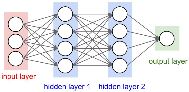
MLP (Multi-layer perception) is layers of neurons

• backpropagate into the weights of all the neurons

• Neuron constructors take in an argument nin (number of inputs)
• Creates a random weight for each of the nin inputs
• for tanh nin random weights are uniformly distributed between -1 and 1
• Neurons also have a single bias b that controls overall trigger happiness
• the __call__ function is basically a nameless function, ie: if you make n = Neuron(2), when you invoke n(x) it is really invoking n.__call__(x)
• we use the __call__ function to implement the forward pass
• the forward pass takes in inputs and computes the dot product + bias
• the activation within the forward pass iterates over the tuples (wi, xi) where wi is each weight and xi is each input. It sums up the product of each tuple and then adds the bias (act)
• finally, we squash the activation and return ie out = act.tanh()
• parameters function returns an array of weights with bias concatenated to the end

Layer class

• a Layer takes in nin, nout
• this creates nout Neurons and each Neuron expects nin inputs
• calling the __call__ function on a Layer will iterate through each Neuron and call the __call__ function for each Neuron (which computes the forward pass)
• parameters function returns an array of neuron parameters for each neuron

MLP class

• an MLM takes in nin and nouts
• nouts is a list that defines the size of all layers in the MLP
• it uses nouts to construct an array of layers where the outputs from one layer become the inputs for the next layer
• the __call__ function iterates through layers and invokes the __call__ function executing the forward pass for each layer of neurons
• parameters function returns array of layer parameters for each layer

By putting the forward pass in the __call__ function, you can invoke this over and over again which once paired with backpropagation will train the weights and biases of the NN

Loss

• loss is a single number that measures how well the Neural Net is performing
• by default, the loss will be high and we want to minimize the loss
• an example loss function would be the mean squared error
• by squaring the mean, you ensure you get a positive number (you could also do abs())
• when the prediction is exactly the target, you get 0 loss
• you compute the mean squared for each prediction - target
• then you sum up the mean squared difference of all the predictions to get the loss
• after computing the loss, calling .backward() will propagate gradients all the way to the beginning input parameters
• the gradients of the input parameters will remain the same, but as we train the NN, the gradients on the weights and biases will be updated nudging closer to values that make better predictions that are more in line with the desired targets

Backpropagation

• in gradient descent, we are thinking of the gradient as a vector pointing in the direction of increased loss
• step size is a small number (ie 0.01, 0.1, 0.05, etc)
• we use small step sizes multiplied by gradients to nudge weights in the direction opposite to the gradient direction ie( -0.01 * p.grad) for each parameter
• continually iterating over forward passes and backward passes and then nudging the weights of the neurons trains the NN
• as the NN gets trained the loss decreases (caveat if you use too high a step size, you can over-correct and get more loss)
• gradient descent is just forward pass, backward pass, update weights
• learning rate and tuning is a subtle art, too low and it can take a long time, too high and it can explode against you

Beware!

most common neural net mistakes you forgot to zero_grad before .backward()

After each forward pass, you need to zero out the gradient so that it doesn't continue to use += operation on the existing gradient. This bug can be subtle on simple NNs, but can be havoc on larger NNs.

To extend autograd functions in Pytorch, define forward and backward pass functions.

Posted In:

jsturgis